Loading

Loading
ShinyItemAnalysis
provides analysis of educational tests (such as admission tests)
and their items including:
This application is based on the free statistical software R and its shiny package.
For all graphical outputs a download button is provided. Moreover, on Reports page HTML or PDF report can be created. Additionaly, all application outputs are complemented by selected R code hence the similar analysis can be run and modified in R.
For demonstration purposes, by default, 20-item dataset
GMAT
from R
difNLR
package is used. Other three datasets are available:
GMAT2
and
Medical 20 DIF
from
difNLR
package and
Medical 100
from
ShinyItemAnalysis
package.
You can change the dataset (and try your own one) on page
Data.
Application can be downloaded as R package from
CRAN.
It is also available online at
Czech Academy of Sciences
![]() .
In case of busy server you can try other mirrors:
Charles University
.
In case of busy server you can try other mirrors:
Charles University
![]() or
shinyapps.io
or
shinyapps.io
![]() .
.
Current version of
ShinyItemAnalysis
available on
CRAN
is 1.2.3.
Version available
online
is 1.2.3.
The newest development version available on
GitHub
is 1.2.3.
See also older versions: 0.1.0, 0.2.0, 1.0.0, 1.1.0.
library(corrplot)
library(CTT)
library(data.table)
library(deltaPlotR)
library(DT)
library(difNLR)
library(difR)
library(ggplot2)
library(grid)
library(gridExtra)
library(knitr)
library(latticeExtra)
library(ltm)
library(mirt)
library(moments)
library(msm)
library(nnet)
library(plotly)
library(psych)
library(psychometric)
library(reshape2)
library(rmarkdown)
library(shiny)
library(shinyjs)
library(stringr)
library(WrightMap)
library(xtable)
If you discover a problem with this application please contact the project maintainer at martinkova(at)cs.cas.cz or use GitHub.
Project was supported by grant funded by Czech Science foundation under number GJ15-15856Y.
This program is free software and you can redistribute it and or modify it under the terms of the GNU GPL 3 as published by the Free Software Foundation. This program is distributed in the hope that it will be useful, but without any warranty; without even the implied warranty of merchantability of fitness for a particular purpose.
For demonstration purposes, 20-item dataset
GMAT
and dataset
GMATkey
from R
difNLR
package are used.
On this page, you may select one of four datasets offered from
difNLR
and
ShinyItemAnalysis
packages or you may upload your own dataset
(see below). To return to demonstration dataset,
refresh this page in your browser
(F5)
.
Used dataset
GMAT
(Martinkova, et al., 2017)
is generated based on parameters of real Graduate Management
Admission Test (GMAT) data set (Kingston et al., 1985). However, first two items were
generated to function differently in uniform and non-uniform way respectively.
The data set represents responses of 2,000 subjects (1,000 males, 1,000 females) to
multiple-choice test of 20 items. The distribution of total scores is the same for both groups.
See
Martinkova, et al. (2017)
for further discussion.
Dataset
GMAT2
(Drabinova & Martinkova, 2016) is also generated based on parameters of GMAT (Kingston et
al., 1985) from R
difNLR
package . Again, first two items were generated
to function differently in uniform and non-uniform way respectively. The data set
represents responses of 1,000 subjects (500 males, 500 females) to multiple-choice test
of 20 items.
Dataset
MSAT-B
(Drabinova & Martinkova, 2017) is a subset of real Medical School Admission
Test in Biology in Czech Republic. The data set represents responses of 1,407 subjects (484 males,
923 females) to multiple-choice test of 20 items. First item was previously detected as
functioning differently. For more details of item selection see Drabinova & Martinkova (2017).
Dataset can be found in R
difNLR
package.
Dataset
Medical 100
is a real data set of admission test to medical school
from R
ShinyItemAnalysis
package. The data set represents responses of
2,392 subjects (750 males, 1,633 females and 9 subjects without gender specification)
to multiple-choice test of 100 items.
Main data file should contain responses of individual students (rows) to given items (columns). Header may contain item names, no row names should be included. If responses are in unscored ABCD format, the key provides correct response for each item. If responses are scored 0-1, key is vector of 1s.
Group is 0-1 vector, where 0 represents reference group and 1 represents focal group. Its length need to be the same as number of individual students in main dataset. If the group is not provided then it wont be possible to run DIF and DDF detection procedures on DIF/Fairness page.
Criterion variable is either discrete or continuous vector (e.g. future study success or future GPA in case of admission tests) which should be predicted by the measurement. Again, its length needs to be the same as number of individual students in the main dataset. If the criterion variable is not provided then it wont be possible to run validity analysis in Predictive validity section on Validity page.
In all data sets header should be either included or excluded. Columns of dataset are by default renamed to Item and number of particular column. If you want to keep your own names, check box Keep items names below. Missing values in scored dataset are by default evaluated as 0. If you want to keep them as missing, check box Keep missing values below.
Here you can explore uploaded dataset. Rendering of tables can take some time.
For selected cut-score, blue part of histogram shows students with total score above the cut-score, grey column shows students with total score equal to the cut-score and red part of histogram shows students below the cut-score.
Download figurelibrary(difNLR)
data(GMAT)
data <- GMAT[, 1:20]
score <- apply(data, 1, sum) # Total score
# Summary of total score
summary(score)
# Histogram
hist(score, breaks = 0:ncol(data))
Total score
also known as raw score is a total number of correct
answers. It can be used to compare individual score to a norm group, e.g. if the mean
is 12, then individual score can be compared to see if it is below or above this average.
Percentile
indicates the value below which a percentage of observations
falls, e.g. a individual score at the 80th percentile means that the individual score
is the same or higher than the scores of 80% of all respondents.
Success rate
is the percentage of success, e.g. if the maximum points of test
is equal to 20 and individual score is 12 then success rate is 12/20 = 0.6, i.e. 60%.
Z-score
or also standardized score is a linear transformation of total
score with a mean of 0 and with variance of 1. If X is total score, M its mean and SD its
standard deviation then Z-score = (X - M) / SD.
T-score
is transformed Z-score with a mean of 50 and standard deviation
of 10. If Z is Z-score then T-score = (Z * 10) + 50.
library(difNLR)
data(GMAT)
data <- GMAT[, 1:20]
score <- apply(data, 1, sum) # Total score
tosc <- sort(unique(score)) # Levels of total score
perc <- cumsum(prop.table(table(score))) # Percentiles
sura <- 100 * (tosc / max(score)) # Success rate
zsco <- sort(unique(scale(score))) # Z-score
tsco <- 50 + 10 * zsco # T-score
Polychoric correlation heat map is a correlation plot which displays a polychoric correlations of items. The size and shade of circles indicate how much the items are correlated (larger and darker circle means larger correlation). The color of circles indicates in which way the items are correlated - blue color shows possitive correlation and red color shows negative correlation.
Download figureA scree plot displays the eigenvalues associated with an component or a factor in descending order versus the number of the component or factor.
Download figurelibrary(corrplot)
library(difNLR)
library(psych)
data(GMAT)
data <- GMAT[, 1:20]
# Correlation plot
corP <- polychoric(data)
corrplot(corP$rho)
corP$rho # Correlation matrix
# Scree plot
plot(1:length(eigen(corP$rho)$values), eigen(corP$rho)$values,
                                            ylab = "Eigen value", xlab = "Component Number")
lines(1:length(eigen(corP$rho)$values), eigen(corP$rho)$values)
eigen(corP$rho) # Eigen values and vectors
This section requires criterion variable (e.g. future study success or future GPA in case of admission tests) which should be predicted by the measurement. This outcome variable can be uploaded in Data section. Then you can explore how data predict this variable.
Total scores are plotted according to criterion variable. Boxplot or scatterplot is displayed depending on outcome variable - whether it is discrete or continuous. Scatterplot is provided with red linear regression line.
Download figureTest for association between total score and criterion variable is based on Spearman`s \(\rho\). This rank-based measure has been recommended if bivariate normal distribution is not guaranteed. The null hypothesis is that correlation is 0.
library(ShinyItemAnalysis)
library(difNLR)
data(GMAT)
data01 <- GMAT[, 1:20]
score <- apply(data01, 1, sum)
criterion <- GMAT[, "criterion"]
# Descriptive plots
### boxplot
boxplot(criterion ~ score)
### scatterplot
plot(criterion ~ score)
abline(lm(criterion ~ score), col = "red")
# Correlation
cor.test(criterion, score, method = "spearman", exact = F)
This section requires criterion variable (e.g. future study success or future GPA in case of admission tests) which should be predicted by the measurement. This outcome variable can be uploaded in Data section. Here you can explore how data predict this variable item by item.
In distractor analysis based on criterion variable, we are interested in how test takers select the correct answer and how the distractors (wrong answers) with respect to group based on criterion variable.
With option Combinations all item selection patterns are plotted (e.g. AB, ACD, BC). With option Distractors answers are splitted into distractors (e.g. A, B, C, D).
Test for association between total score and criterion variable is based on Spearman`s \(\rho\). This rank-based measure has been recommended if bivariate normal distribution is not guaranteed. The null hypothesis is that correlation is 0.
library(ShinyItemAnalysis)
library(difNLR)
data("GMAT", "GMATtest", "GMATkey")
data <- GMATtest[, 1:20]
data01 <- GMAT[, 1:20]
key <- GMATkey
criterion <- GMAT[, "criterion"]
# Distractor plot for item 1 and 3 groups
plotDistractorAnalysis(data, key, num.groups = 3, item = 1, matching = criterion)
# Correlation for item 1
cor.test(criterion, data01[, 1], method = "spearman", exact = F)
Traditional item analysis uses proportions of correct answers or correlations to estimate item properties.
Displayed is difficulty (red) and discrimination (blue)
for all items. Items are ordered by difficulty.
Difficulty
of items is estimated as percent of students who
answered correctly to that item.
Discrimination
is by default described by difference of percent correct
in upper and lower third of students (Upper-Lower Index, ULI). By rule of
thumb it should not be lower than 0.2 (borderline in the plot), except for
very easy or very difficult items. Discrimination can be customized (see also Martinkova, Stepanek, et al.
(2017)) by changing number of groups and by changing which groups should be compared:
Chronbach's alpha is an estimate of the reliability of a psychometric test. It is a function of the number of items in a test, the average covariance between item-pairs, and the variance of the total score (Cronbach, 1951).
library(difNLR)
library(psych)
library(psychometric)
library(ShinyItemAnalysis)
data(GMAT)
data <- GMAT[, 1:20]
# Difficulty and discrimination plot
DDplot(data, k = 3, l = 1, u = 3)
# Cronbach alpha
psych::alpha(data)
# Table
tab <- round(data.frame(item.exam(data, discr = TRUE)[, c(4, 1, 5, 2, 3)],
                                          psych::alpha(data)$alpha.drop[, 1], gDiscrim(data, k = 3, l = 1, u = 3)), 2)
colnames(tab) <- c("Difficulty", "SD", "Dsicrimination ULI", "Discrimination RIT", "Discrimination RIR", "Alpha Drop", "Customized Discrimination")
tab
In distractor analysis, we are interested in how test takers select the correct answer and how the distractors (wrong answers) were able to function effectively by drawing the test takers away from the correct answer.
With option Combinations all item selection patterns are plotted (e.g. AB, ACD, BC). With option Distractors answers are splitted into distractors (e.g. A, B, C, D).
library(difNLR)
library(ShinyItemAnalysis)
data(GMATtest)
data <- GMATtest[, colnames(GMATtest) != "group"]
data(GMATkey)
key <- GMATkey
# Combinations - plot for item 1 and 3 groups
plotDistractorAnalysis(data, key, num.group = 3, item = 1,
                                          multiple.answers = T)
# Distractors - plot for item 1 and 3 groups
plotDistractorAnalysis(data, key, num.group = 3, item = 1,
                                          multiple.answers = F)
# Table with counts and margins - item 1 and 3 groups
DA <- DistractorAnalysis(data, key, num.groups = 3)[[1]]
dcast(as.data.frame(DA), response ~ score.level, sum, margins = T, value.var = "Freq")
# Table with proportions - item 1 and 3 groups
DistractorAnalysis(data, key, num.groups = 3, p.table = T)[[1]]
tab
Various regression models may be fitted to describe item properties in more detail. Logistic regression can model dependency of probability of correct answer on total score by S-shaped logistic curve. Parameter b0 describes horizontal position of the fitted curve, parameter b1 describes its slope.
Points represent proportion of correct answer with respect to total score. Their size is determined by count of respondents who answered item correctly.
library(difNLR)
data(GMAT)
data <- GMAT[, 1:20]
score <- apply(data, 1, sum)
# Logistic model for item 1
fit <- glm(data[, 1] ~ score, family = binomial)
# Coefficients
coef(fit)
# Function for plot
fun <- function(x, b0, b1){exp(b0 + b1 * x) / (1 + exp(b0 + b1 * x))}
# Plot of estimated curve
curve(fun(x, b0 = coef(fit)[1], b1 = coef(fit)[2]), 0, 20,
                                          xlab = "Total score",
                                          ylab = "Probability of correct answer",
                                          ylim = c(0, 1))
Various regression models may be fitted to describe item properties in more detail. Logistic regression can model dependency of probability of correct answer on standardized total score (Z-score) by S-shaped logistic curve. Parameter b0 describes horizontal position of the fitted curve (difficulty), parameter b1 describes its slope at inflection point (discrimination).
Points represent proportion of correct answer with respect to standardized total score. Their size is determined by count of respondents who answered item correctly.
library(difNLR)
data(GMAT)
data <- GMAT[, 1:20]
stand.score <- scale(apply(data, 1, sum))
# Logistic model for item 1
fit <- glm(data[, 1] ~ stand.score, family = binomial)
# Coefficients
coef(fit)
# Function for plot
fun <- function(x, b0, b1){exp(b0 + b1 * x) / (1 + exp(b0 + b1 * x))}
# Plot of estimated curve
curve(fun(x, b0 = coef(fit)[1], b1 = coef(fit)[2]), -3, 3,
                                          xlab = "Standardized total score",
                                          ylab = "Probability of correct answer",
                                          ylim = c(0, 1))
Various regression models may be fitted to describe item properties in more detail. Logistic regression can model dependency of probability of correct answer on standardized total score (Z-score) by s-shaped logistic curve. Note change in parametrization - the IRT parametrization used here corresponds to the parametrization used in IRT models. Parameter b describes horizontal position of the fitted curve (difficulty), parameter a describes its slope at inflection point (discrimination).
Points represent proportion of correct answer with respect to standardized total score. Their size is determined by count of respondents who answered item correctly.
library(difNLR)
data(GMAT)
data <- GMAT[, 1:20]
stand.score <- scale(apply(data, 1, sum))
# Logistic model for item 1
fit <- glm(data[, 1] ~ stand.score, family = binomial)
# Coefficients - tranformation
coef <- c(a = coef(fit)[2], b = - coef(fit)[1] / coef(fit)[2])
coef
# Function for plot
fun <- function(x, a, b){exp(a * (x - b)) / (1 + exp(a * (x - b)))}
# Plot of estimated curve
curve(fun(x, a = coef[1], b = coef[2]), -3, 3,
                                          xlab = "Standardized total score",
                                          ylab = "Probability of correct answer",
                                          ylim = c(0, 1))
Various regression models may be fitted to describe item properties in more detail. Nonlinear regression can model dependency of probability of correct answer on standardized total score (Z-score) by s-shaped logistic curve. The IRT parametrization used here corresponds to the parametrization used in IRT models. Parameter b describes horizontal position of the fitted curve (difficulty), parameter a describes its slope at inflection point (discrimination). This model allows for nonzero lower left asymptote c (pseudo-guessing).
Points represent proportion of correct answer with respect to standardized total score. Their size is determined by count of respondents who answered item correctly.
library(difNLR)
data(GMAT)
Data <- GMAT[, 1:20]
stand.score <- scale(apply(Data, 1, sum))
# NLR model for item 1
fun <- function(x, a, b, c){c + (1 - c) * exp(a * (x - b)) / (1 + exp(a * (x - b)))}
fit <- nls(data[, 1] ~ fun(stand.score, a, b, c), algorithm = "port",
                                          start = startNLR(data, GMAT[, "group"], model = "3PLcg")[1, 1:3])
# Coefficients
coef(fit)
# Plot of estimated curve
curve(fun(x, a = coef(fit)[1], b = coef(fit)[2], c = coef(fit)[3]), -3, 3,
                                          xlab = "Standardized total score",
                                          ylab = "Probability of correct answer",
                                          ylim = c(0, 1))
Here you can compare classic 2PL logistic regression model to non-linear model item by item using some information criterions:
Another approach to nested models can be likelihood ratio chi-squared test. Significance level is set to 0.05. As tests are performed item by item, it is possible to use multiple comparison correction method.
Rows BEST indicate which model has the lowest value of criterion, or is the largest significant model by likelihood ratio test.
library(difNLR)
data(GMAT)
Data <- GMAT[, 1:20]
stand.score <- scale(apply(Data, 1, sum))
# Fitting models
fun <- function(x, a, b, c){c + (1 - c) * exp(a * (x - b)) / (1 + exp(a * (x - b)))}
# 2PL model for item 1
fit2PL <- nls(Data[, 1] ~ fun(stand.score, a, b, c = 0), algorithm = "port",
                                          start = startNLR(Data, GMAT[, "group"], model = "3PLcg")[1, 1:2])
# 3PL model for item 1
fit3PL <- nls(Data[, 1] ~ fun(stand.score, a, b, c), algorithm = "port",
                                          start = startNLR(Data, GMAT[, "group"], model = "3PLcg")[1, 1:3])
# Comparison
AIC(fit2PL); AIC(fit3PL)
BIC(fit2PL); BIC(fit3PL)
LRstat <- -2 * (sapply(fit2PL, logLik) - sapply(fit3PL, logLik))
LRdf <- 1
LRpval <- 1 - pchisq(LRstat, LRdf)
LRpval <- p.adjust(LRpval, method = "BH")
Various regression models may be fitted to describe item properties in more detail. Multinomial regression allows for simultaneous modelling of probability of choosing given distractors on standardized total score (Z-score).
Points represent proportion of selected option with respect to standardized total score. Their size is determined by count of respondents who selected given option.
library(difNLR)
library(nnet)
data(GMAT)
data.scored <- GMAT[, 1:20]
stand.score <- scale(apply(data, 1, sum))
data(GMATtest)
data <- GMATtest[, colnames(GMATtest) != "group"]
data(GMATkey)
key <- GMATkey
# multinomial model for item 1
fit <- multinom(relevel(data[, 1], ref = paste(key[1])) ~ stand.score)
# Coefficients
coef(fit)
Item Response Theory (IRT) models are mixed-effect regression models in which student ability (theta) is assumed to be a random effect and is estimated together with item paramters. Ability (theta) is often assumed to follow normal distibution.
In Rasch IRT model (Rasch, 1960), all items are assumed to have the same slope in inflection point – the same discrimination a which is fixed to value of 1. Items can differ in location of their inflection point – in item difficulty b.
Estimates of parameters are completed by SX2 item fit statistics (Ames & Penfield, 2015). SX2 is computed only when no missing data are present. In such a case consider using imputed dataset!
Wright map (Wilson, 2005; Wright & Stone, 1979), also called item-person map, is a graphical tool to display person estimates and item parameters. The person side (left) represents histogram of estimated knowledge of students. The item side (right) displays estimates of difficulty of particular items.
Download figurelibrary(difNLR)
library(mirt)
library(WrightMap)
data(GMAT)
data <- GMAT[, 1:20]
# Model
fit <- mirt(data, model = 1, itemtype = "Rasch", SE = T)
# Item Characteristic Curves
plot(fit, type = "trace", facet_items = F)
# Item Information Curves
plot(fit, type = "infotrace", facet_items = F)
# Test Information Function
plot(fit, type = "infoSE")
# Coefficients
coef(fit, simplify = TRUE)
coef(fit, IRTpars = TRUE, simplify = TRUE)
# Item fit statistics
itemfit(fit)
# Factor scores vs Standardized total scores
fs <- as.vector(fscores(fit))
sts <- as.vector(scale(apply(data, 1, sum)))
plot(fs ~ sts)
# Wright Map
b <- sapply(1:ncol(data), function(i) coef(fit)[[i]][, "d"])
wrightMap(fs, b, item.side = itemClassic)
Item Response Theory (IRT) models are mixed-effect regression models in which student ability (theta) is assumed to be a random effect and is estimated together with item paramters. Ability (theta) is often assumed to follow normal distibution.
In 1PL IRT model , all items are assumed to have the same slope in inflection point – the same discrimination a . Items can differ in location of their inflection point – in item difficulty b.
Estimates of parameters are completed by SX2 item fit statistics (Ames & Penfield, 2015). SX2 is computed only when no missing data are present. In such a case consider using imputed dataset!
Wright map (Wilson, 2005; Wright & Stone, 1979), also called item-person map, is a graphical tool to display person estimates and item parameters. The person side (left) represents histogram of estimated knowledge of students. The item side (right) displays estimates of difficulty of particular items.
Download figurelibrary(difNLR)
library(mirt)
library(WrightMap)
data(GMAT)
data <- GMAT[, 1:20]
# Model
fit <- mirt(data, model = 1, itemtype = "2PL", constrain = list((1:ncol(data)) + seq(0, (ncol(data) - 1)*3, 3)), SE = T)
# Item Characteristic Curves
plot(fit, type = "trace", facet_items = F)
# Item Information Curves
plot(fit, type = "infotrace", facet_items = F)
# Test Information Function
plot(fit, type = "infoSE")
# Coefficients
coef(fit, simplify = TRUE)
coef(fit, IRTpars = TRUE, simplify = TRUE)
# Item fit statistics
itemfit(fit)
# Factor scores vs Standardized total scores
fs <- as.vector(fscores(fit))
sts <- as.vector(scale(apply(data, 1, sum)))
plot(fs ~ sts)
# Wright Map
b <- sapply(1:ncol(data), function(i) coef(fit)[[i]][, "d"])
wrightMap(fs, b, item.side = itemClassic)
# You can also use ltm library for IRT models
library(difNLR)
library(ltm)
data(GMAT)
data <- GMAT[, 1:20]
# Model
fit <- rasch(data)
# for Rasch model use
# fit <- rasch(data, constraint = cbind(ncol(data) + 1, 1))
# Item Characteristic Curves
plot(fit)
# Item Information Curves
plot(fit, type = "IIC")
# Test Information Function
plot(fit, items = 0, type = "IIC")
# Coefficients
coef(fit)
# Factor scores vs Standardized total scores
df1 <- ltm::factor.scores(fit, return.MIvalues = T)$score.dat
FS <- as.vector(df1[, "z1"])
df2 <- df1
df2$Obs <- df2$Exp <- df2$z1 <- df2$se.z1 <- NULL
STS <- as.vector(scale(apply(df2, 1, sum)))
df <- data.frame(FS, STS)
plot(FS ~ STS, data = df,
                                          xlab = "Standardized total score",
                                          ylab = "Factor score")
Item Response Theory (IRT) models are mixed-effect regression models in which student ability (theta) is assumed to be a random effect and is estimated together with item paramters. Ability (theta) is often assumed to follow normal distibution.
2PL IRT model allows for different slopes in inflection point – different discriminations a. Items can also differ in location of their inflection point – in item difficulty b.
Estimates of parameters are completed by SX2 item fit statistics (Ames & Penfield, 2015). SX2 is computed only when no missing data are present. In such a case consider using imputed dataset!
library(difNLR)
library(mirt)
data(GMAT)
data <- GMAT[, 1:20]
# Model
fit <- mirt(data, model = 1, itemtype = "2PL", SE = T)
# Item Characteristic Curves
plot(fit, type = "trace", facet_items = F)
# Item Information Curves
plot(fit, type = "infotrace", facet_items = F)
# Test Information Function
plot(fit, type = "infoSE")
# Coefficients
coef(fit, simplify = TRUE)
coef(fit, IRTpars = TRUE, simplify = TRUE)
# Item fit statistics
itemfit(fit)
# Factor scores vs Standardized total scores
fs <- as.vector(fscores(fit))
sts <- as.vector(scale(apply(data, 1, sum)))
plot(fs ~ sts)
# You can also use ltm library for IRT models
library(difNLR)
library(ltm)
data(GMAT)
data <- GMAT[, 1:20]
# Model
fit <- ltm(data ~ z1, IRT.param = TRUE)
# Item Characteristic Curves
plot(fit)
# Item Information Curves
plot(fit, type = "IIC")
# Test Information Function
plot(fit, items = 0, type = "IIC")
# Coefficients
coef(fit)
# Factor scores vs Standardized total scores
df1 <- ltm::factor.scores(fit, return.MIvalues = T)$score.dat
FS <- as.vector(df1[, "z1"])
df2 <- df1
df2$Obs <- df2$Exp <- df2$z1 <- df2$se.z1 <- NULL
STS <- as.vector(scale(apply(df2, 1, sum)))
df <- data.frame(FS, STS)
plot(FS ~ STS, data = df,
                                          xlab = "Standardized total score",
                                          ylab = "Factor score")
Item Response Theory (IRT) models are mixed-effect regression models in which student ability (theta) is assumed to be a random effect and is estimated together with item paramters. Ability (theta) is often assumed to follow normal distibution.
3PL IRT model allows for different discriminations of items a, different item difficulties b, and allows also for nonzero left asymptote – pseudo-guessing c.
Estimates of parameters are completed by SX2 item fit statistics (Ames & Penfield, 2015). SX2 is computed only when no missing data are present. In such a case consider using imputed dataset!
library(difNLR)
library(mirt)
data(GMAT)
data <- GMAT[, 1:20]
# Model
fit <- mirt(data, model = 1, itemtype = "3PL", SE = T)
# Item Characteristic Curves
plot(fit, type = "trace", facet_items = F)
# Item Information Curves
plot(fit, type = "infotrace", facet_items = F)
# Test Information Function
plot(fit, type = "infoSE")
# Coefficients
coef(fit, simplify = TRUE)
coef(fit, IRTpars = TRUE, simplify = TRUE)
# Item fit statistics
itemfit(fit)
# Factor scores vs Standardized total scores
fs <- as.vector(fscores(fit))
sts <- as.vector(scale(apply(data, 1, sum)))
plot(fs ~ sts)
# You can also use ltm library for IRT models
library(difNLR)
library(ltm)
data(GMAT)
data <- GMAT[, 1:20]
# Model
fit <- tpm(data, IRT.param = TRUE)
# Item Characteristic Curves
plot(fit)
# Item Information Curves
plot(fit, type = "IIC")
# Test Information Function
plot(fit, items = 0, type = "IIC")
# Coefficients
coef(fit)
# Factor scores vs Standardized total scores
df1 <- ltm::factor.scores(fit, return.MIvalues = T)$score.dat
FS <- as.vector(df1[, "z1"])
df2 <- df1
df2$Obs <- df2$Exp <- df2$z1 <- df2$se.z1 <- NULL
STS <- as.vector(scale(apply(df2, 1, sum)))
df <- data.frame(FS, STS)
plot(FS ~ STS, data = df,
                                          xlab = "Standardized total score",
                                          ylab = "Factor score")
Item Response Theory (IRT) models are mixed-effect regression models in which student ability (theta) is assumed to be a random effect and is estimated together with item paramters. Ability (theta) is often assumed to follow normal distibution.
IRT models can be compared by several information criterions:
Another approach to compare IRT models can be likelihood ratio chi-squared test. Significance level is set to 0.05.
Row BEST indicates which model has the lowest value of criterion, or is the largest significant model by likelihood ratio test.
library(difNLR)
library(mirt)
data(GMAT)
data <- GMAT[, 1:20]
# 1PL IRT model
fit1PL <- mirt(data, model = 1, itemtype = "3PL", SE = T)
# 2PL IRT model
fit2PL <- mirt(data, model = 1, itemtype = "2PL")
# 3PL IRT model
fit3PL <- mirt(data, model = 1, itemtype = "3PL")
# Comparison
anova(fit1PL, fit2PL)
anova(fit2PL, fit3PL)
The nominal response model (NRM) was introduced by Bock (1972) as a way to model responses to items with two or more nominal categories. This model is suitable for multiple-choice items with no particular ordering of distractors. The correct answer represent the highest category, in terms of the measured latent trait.
library(difNLR)
library(mirt)
data(GMAT)
data <- GMAT[, 1:20]
# Model
fit <- mirt(data, model = 1, itemtype = "nominal")
# Item Characteristic Curves
plot(fit, type = "trace", facet_items = F)
# Item Information Curves
plot(fit, type = "infotrace", facet_items = F)
# Test Information Function
plot(fit, type = "infoSE")
# Coefficients
coef(fit, simplify = TRUE)
coef(fit, IRTpars = TRUE, simplify = TRUE)
# Factor scores vs Standardized total scores
fs <- as.vector(fscores(fit))
sts <- as.vector(scale(apply(data, 1, sum)))
plot(fs ~ sts)
Here you can explore behaviour of two item characteristic curves \(\mathrm{P}\left(\theta\right)\) and their item information functions \(\mathrm{I}\left(\theta\right)\) in 4PL IRT model.
Select parameters a (discrimination), b (difficulty), c (guessing) and d (inattention). By constraining a = 1, c = 0, d = 1 you get Rasch model. With option c = 0 and d = 1 you get 2PL model and with option d = 1 3PL model.
When you set different curve parameters, you can follow a phenomenon called Differential Item Functioning (DIF). See further section for more information.
DIF is not about total scores! Two groups may have the same distribution of total scores, yet, some item may function differently for two groups. Also, one of the groups may have signifficantly lower total score, yet, it may happen that there is no DIF item!
For selected cut-score, blue part of histogram shows students with total score above the cut-score, grey column shows students with Total Score equal to cut-score and red part of histogram shows students below the cut-score.
library(difNLR)
data <- GMAT[, 1:20]
group <- GMAT[, "group"]
# Summary table
sc_zero <- apply(data[group == 0, ], 1, sum); summary(sc_zero) # total scores of reference group
sc_one <- apply(data[group == 1, ], 1, sum); summary(sc_one) # total scores of focal group
# Histograms
hist(sc_zero, breaks = 0:20)
hist(sc_one, breaks = 0:20)
Delta plot (Angoff & Ford, 1973) compares the proportions of correct answers per item in the two groups. It displays non-linear transformation of these proportions using quantiles of standard normal distributions (so called delta scores) for each item for the two genders in a scatterplot called diagonal plot or delta plot (see Figure). Item is under suspicion of DIF if the delta point considerably departs from the diagonal. The detection threshold is either fixed to value 1.5 or based on bivariate normal approximation (Magis & Facon, 2012).
library(deltaPlotR)
library(difNLR)
data(GMAT)
data <- GMAT[, 1:20]
group <- GMAT[, "group"]
# Delta scores with fixed threshold
deltascores <- deltaPlot(data.frame(data, group), group = "group",
                                          focal.name = 1, thr = 1.5)
deltascores
# Delta plot
diagPlot(deltascores, thr.draw = T)
# Delta scores with normal threshold
deltascores <- deltaPlot(data.frame(data, group), group = "group",
                                          focal.name = 1, thr = "norm", purify = F)
deltascores
# Delta plot
diagPlot(deltascores, thr.draw = T)
Mantel-Haenszel test is DIF detection method based on contingency tables that are calculated for each level of total score (Mantel & Haenszel, 1959).
library(difNLR)
library(difR)
data(GMAT)
data <- GMAT[, 1:20]
group <- GMAT[, "group"]
# Mantel-Haenszel test
fit <- difMH(Data = data, group = group, focal.name = 1,
                                                     p.adjust.method = "none", purify = F)
fit
Mantel-Haenszel test is DIF detection method based on contingency tables that are calculated for each level of total score (Mantel & Haenszel, 1959).
library(difNLR)
library(difR)
data(GMAT)
data <- GMAT[, 1:20]
group <- GMAT[, "group"]
# Contingency table for item 1 and score 12
df <- data.frame(data[, 1], group)
colnames(df) <- c("Answer", "Group")
df$Answer <- relevel(factor(df$Answer, labels = c("Incorrect", "Correct")), "Correct")
df$Group <- factor(df$Group, labels = c("Reference Group", "Focal Group"))
score <- apply(data, 1, sum)
df <- df[score == 12, ]
tab <- dcast(data.frame(xtabs(~ Group + Answer, data = df)),
                                                     Group ~ Answer,
                                                     value.var = "Freq",
                                                     margins = T,
                                                     fun = sum)
tab
# Mantel-Haenszel estimate of OR
fit <- difMH(Data = data, group = group, focal.name = 1,
                                                     p.adjust.method = "none", purify = F)
fit$alphaMH
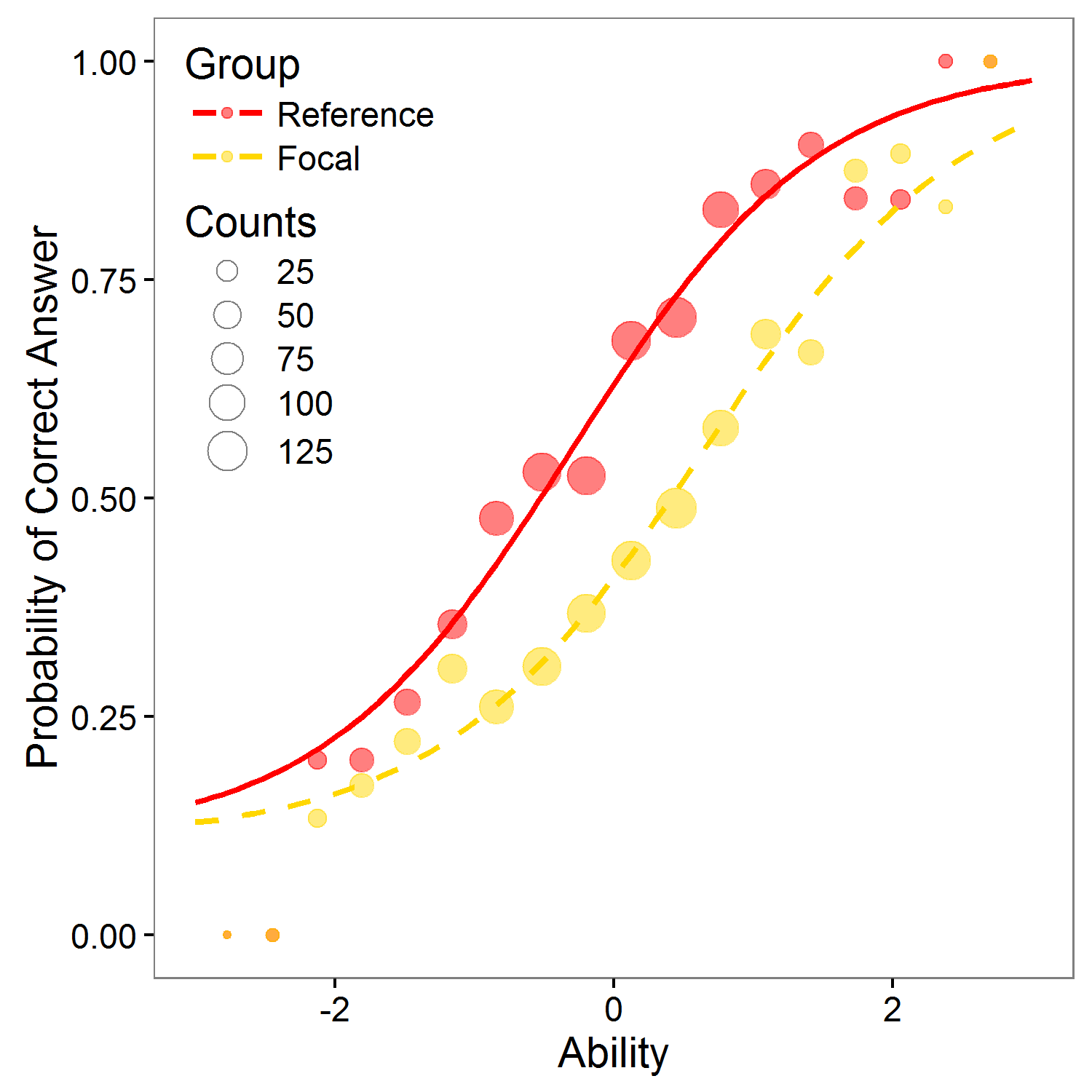
Logistic regression allows for detection of uniform and non-uniform DIF (Swaminathan & Rogers, 1990) by adding a group specific intercept b2 (uniform DIF) and group specific interaction b3 (non-uniform DIF) into model and by testing for their significance.
library(difNLR)
library(difR)
data(GMAT)
data <- GMAT[, 1:20]
group <- GMAT[, "group"]
# Logistic regression DIF detection method
fit <- difLogistic(Data = data, group = group, focal.name = 1,
                                                     type = "both",
                                                     p.adjust.method = "none",
                                                     purify = F)
fit
Logistic regression allows for detection of uniform and non-uniform DIF by adding a group specific intercept b2 (uniform DIF) and group specific interaction b3 (non-uniform DIF) into model and by testing for their significance.
Points represent proportion of correct answer with respect to standardized total score. Their size is determined by count of respondents who answered item correctly.
NOTE: Plots and tables are based on DIF logistic procedure without any correction method.
library(difNLR)
library(difR)
data(GMAT)
data <- GMAT[, 1:20]
group <- GMAT[, "group"]
# Logistic regression DIF detection method
fit <- difLogistic(Data = data, group = group, focal.name = 1,
                                                     type = "both",
                                                     p.adjust.method = "none", purify = F)
fit
# Plot of characteristic curve for item 1
plotDIFLogistic(data, group,
                                                     type = "both",
                                                     item =  1,
                                                     IRT = F,
                                                     p.adjust.method = "none",
                                                     purify = F)
# Coefficients
fit$logitPar
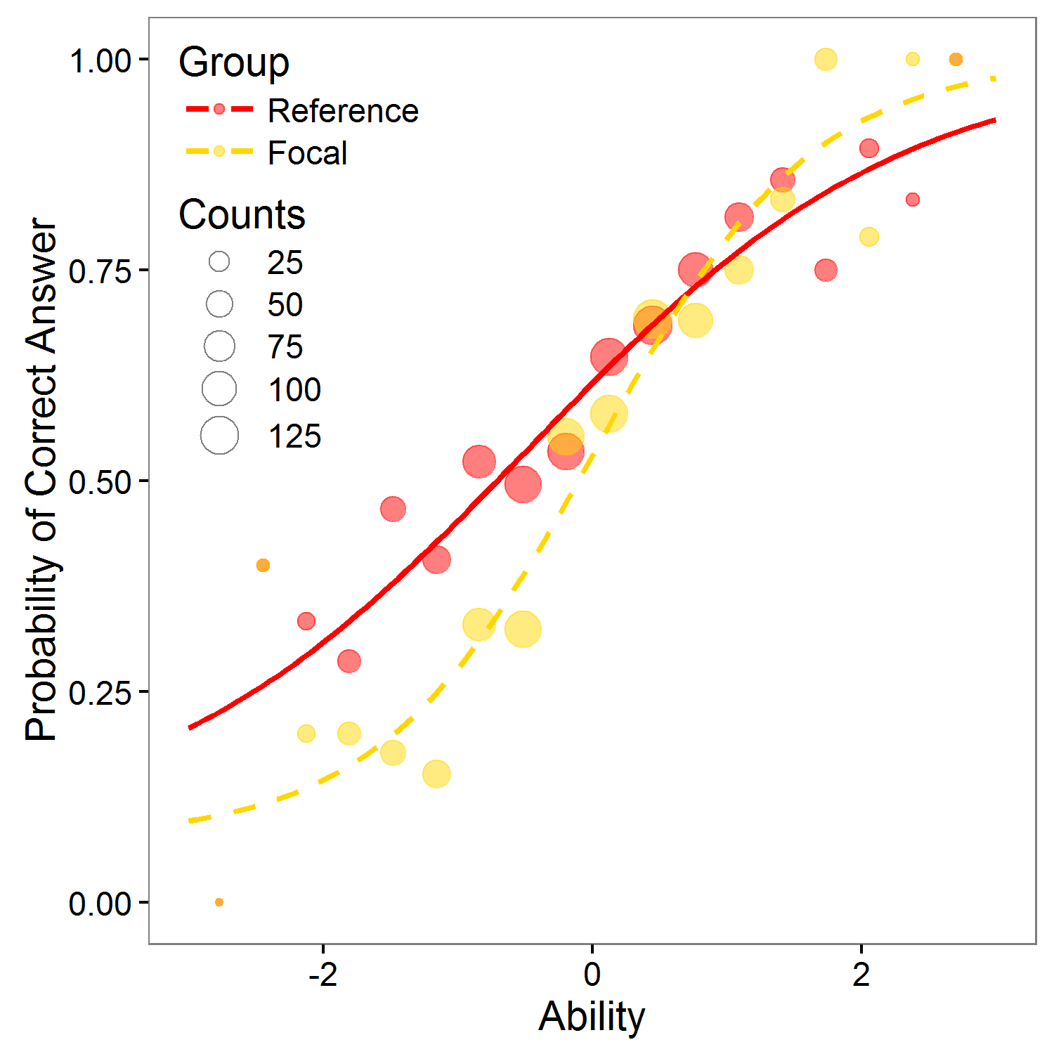
Logistic regression allows for detection of uniform and non-uniform DIF (Swaminathan & Rogers, 1990) by adding a group specific intercept bDIF (uniform DIF) and group specific interaction aDIF (non-uniform DIF) into model and by testing for their significance.
library(difNLR)
library(difR)
data(GMAT)
data <- GMAT[, 1:20]
group <- GMAT[, "group"]
scaled.score <- scale(score)
# Logistic regression DIF detection method
fit <- difLogistic(Data = data, group = group, focal.name = 1,
                                                     type = "both",
                                                     match = scaled.score,
                                                     p.adjust.method = "none",
                                                     purify = F)
fit
Logistic regression allows for detection of uniform and non-uniform DIF by adding a group specific intercept bDIF (uniform DIF) and group specific interaction aDIF (non-uniform DIF) into model and by testing for their significance.
Points represent proportion of correct answer with respect to standardized total score. Their size is determined by count of respondents who answered item correctly.
NOTE: Plots and tables are based on DIF logistic procedure without any correction method.
library(difNLR)
library(difR)
data(GMAT)
data <- GMAT[, 1:20]
group <- GMAT[, "group"]
scaled.score <- scale(score)
# Logistic regression DIF detection method
fit <- difLogistic(Data = data, group = group, focal.name = 1,
                                                     type = "both",
                                                     match = scaled.score,
                                                     p.adjust.method = "none",
                                                     purify = F)
fit
# Plot of characteristic curve for item 1
plotDIFLogistic(data, group,
                                                     type = "both",
                                                     item =  1,
                                                     IRT = T,
                                                     p.adjust.method = "BH")
# Coefficients for item 1 - recalculation
coef_old <- fit$logitPar[1, ]
coef <- c()
# a = b1, b = -b0/b1, adif = b3, bdif = -(b1b2-b0b3)/(b1(b1+b3))
coef[1] <- coef_old[2]
coef[2] <- -(coef_old[1] / coef_old[2])
coef[3] <- coef_old[4]
coef[4] <- -(coef_old[2] * coef_old[3] + coef_old[1] * coef_old[4] ) /
                                                     (coef_old[2] * (coef_old[2] + coef_old[4]))
Nonlinear regression model allows for nonzero lower asymptote - pseudoguessing c. Similarly to logistic regression, also nonlinear regression allows for detection of uniform and non-uniform DIF by adding a group specific intercept bDIF (uniform DIF) and group specific interaction aDIF (non-uniform DIF) into the model and by testing for their significance.
library(difNLR)
data(GMAT)
Data <- GMAT[, 1:20]
group <- GMAT[, "group"]
# Nonlinear regression DIF method
fit <- difNLR(Data = Data, group = group, focal.name = 1,
                                                     model = "3PLcg", type = "both", p.adjust.method = "none")
fit
Nonlinear regression model allows for nonzero lower asymptote - pseudoguessing c. Similarly to logistic regression, also nonlinear regression allows for detection of uniform and non-uniform DIF (Drabinova & Martinkova, 2016) by adding a group specific intercept bDIF (uniform DIF) and group specific interaction aDIF (non-uniform DIF) into the model and by testing for their significance.
Points represent proportion of correct answer with respect to standardized total score. Their size is determined by count of respondents who answered item correctly.
library(difNLR)
data(GMAT)
Data <- GMAT[, 1:20]
group <- GMAT[, "group"]
# Nonlinear regression DIF method
fit <- difNLR(Data = Data, group = group, focal.name = 1,
                                                     model = "3PLcg", type = "both", p.adjust.method = "none")
# Plot of characteristic curve of item 1
plot(fit, item = 1)
# Coefficients
fit$nlrPAR
Lord test (Lord, 1980) is based on IRT model (1PL, 2PL, or 3PL with the same guessing). It uses the difference between item parameters for the two groups to detect DIF. In statistical terms, Lord statistic is equal to Wald statistic.
library(difNLR)
library(difR)
data(GMAT)
data <- GMAT[, 1:20]
group <- GMAT[, "group"]
# 2PL IRT MODEL
fit <- difLord(Data = data, group = group, focal.name = 1,
                                                     model = "2PL",
                                                     p.adjust.method = "none", purify = F)
fit
Lord test (Lord, 1980) is based on IRT model (1PL, 2PL, or 3PL with the same guessing). It uses the difference between item parameters for the two groups to detect DIF. In statistical terms, Lord statistic is equal to Wald statistic.
NOTE: Plots and tables are based on larger DIF IRT model.
library(difNLR)
library(difR)
data(GMAT)
data <- GMAT[, 1:20]
group <- GMAT[, "group"]
# 2PL IRT MODEL
fit <- difLord(Data = data, group = group, focal.name = 1,
                                                     model = "2PL",
                                                     p.adjust.method = "none", purify = F)
fit
# Coefficients for item 1
tab_coef <- fit$itemParInit[c(1, ncol(data) + 1), 1:2]
# Plot of characteristic curve of item 1
plotDIFirt(parameters = tab_coef, item = 1)
Raju test (Raju, 1988, 1990) is based on IRT model (1PL, 2PL, or 3PL with the same guessing). It uses the area between the item charateristic curves for the two groups to detect DIF.
library(difNLR)
library(difR)
data(GMAT)
data <- GMAT[, 1:20]
group <- GMAT[, "group"]
# 2PL IRT MODEL
fit <- difRaju(Data = data, group = group, focal.name = 1,
                                                     model = "2PL",
                                                     p.adjust.method = "none", purify = F)
fit
Raju test (Raju, 1988, 1990) is based on IRT model (1PL, 2PL, or 3PL with the same guessing). It uses the area between the item charateristic curves for the two groups to detect DIF.
NOTE: Plots and tables are based on larger DIF IRT model.
library(difNLR)
library(difR)
data(GMAT)
data <- GMAT[, 1:20]
group <- GMAT[, "group"]
# 2PL IRT MODEL
fit <- difRaju(Data = data, group = group, focal.name = 1,
                                                     model = "2PL",
                                                     p.adjust.method = "none", purify = F)
fit
# Coefficients for item 1
tab_coef <- fit$itemParInit[c(1, ncol(data) + 1), 1:2]
# Plot of characteristic curve of item 1
plotDIFirt(parameters = tab_coef, item = 1, test = "Raju")
Differential Distractor Functioning (DDF) occurs when people from different groups but with the same knowledge have different probability of selecting at least one distractor choice. DDF is here examined by Multinomial Log-linear Regression model with Z-score and group membership as covariates.
For K possible test choices is the probability of the correct answer for person i with standardized total score Z and group membership G in item j given by the following equation:
$$\mathrm{P}(Y_{ij} = K|Z_i, G_i, b_{jl0}, b_{jl1}, b_{jl2}, b_{jl3}, l = 1, \dots, K-1) = \frac{1}{1 + \sum_l e^{\left( b_{il0} + b_{il1} Z + b_{il2} G + b_{il3} Z:G\right)}}$$The probability of choosing distractor k is then given by:
$$\mathrm{P}(Y_{ij} = k|Z_i, G_i, b_{jl0}, b_{jl1}, b_{jl2}, b_{jl3}, l = 1, \dots, K-1) = \frac{e^{\left( b_{jk0} + b_{jk1} Z_i + b_{jk2} G_i + b_{jk3} Z_i:G_i\right)}} {1 + \sum_l e^{\left( b_{jl0} + b_{jl1} Z_i + b_{jl2} G_i + b_{jl3} Z_i:G_i\right)}}$$library(difNLR)
data(GMATtest, GMATkey)
Data <- GMATtest[, 1:20]
group <- GMATtest[, "group"]
key <- GMATkey
# DDF with difNLR package
fit <- ddfMLR(Data, group, focal.name = 1, key, type = "both",
                                                     p.adjust.method = "none")
fit
Differential Distractor Functioning (DDF) occurs when people from different groups but with the same knowledge have different probability of selecting at least one distractor choice. DDF is here examined by Multinomial Log-linear Regression model with Z-score and group membership as covariates.
Points represent proportion of selected answer with respect to standardized total score. Size of points is determined by count of respondents who chose particular answer.
library(difNLR)
data(GMATtest, GMATkey)
Data <- GMATtest[, 1:20]
group <- GMATtest[, "group"]
key <- GMATkey
# DDF with difNLR package
fit <- ddfMLR(Data, group, focal.name = 1, key, type = "both",
                                                     p.adjust.method = "none")
# Estimated coefficients of item 1
fit$mlrPAR[[1]]
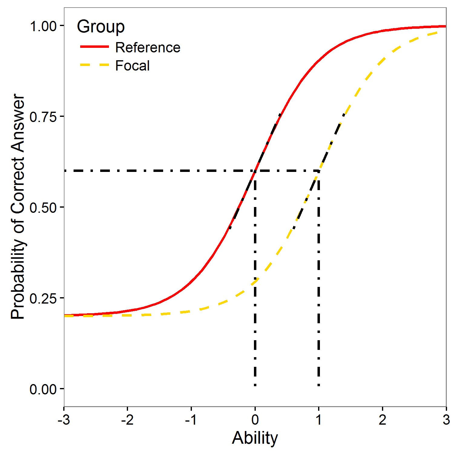
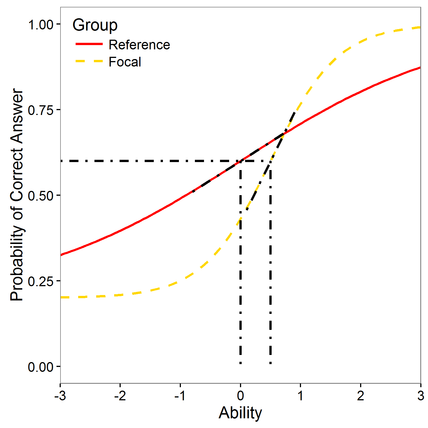
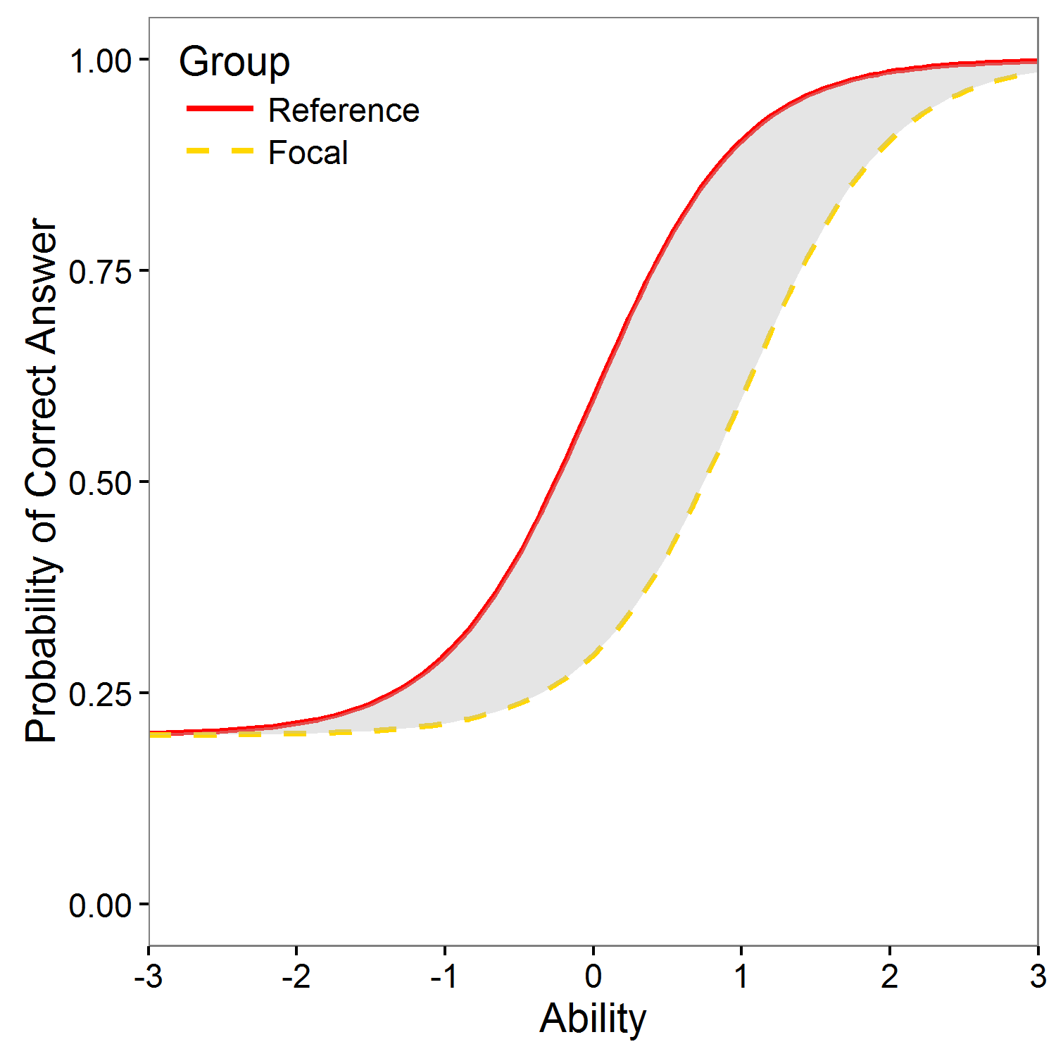
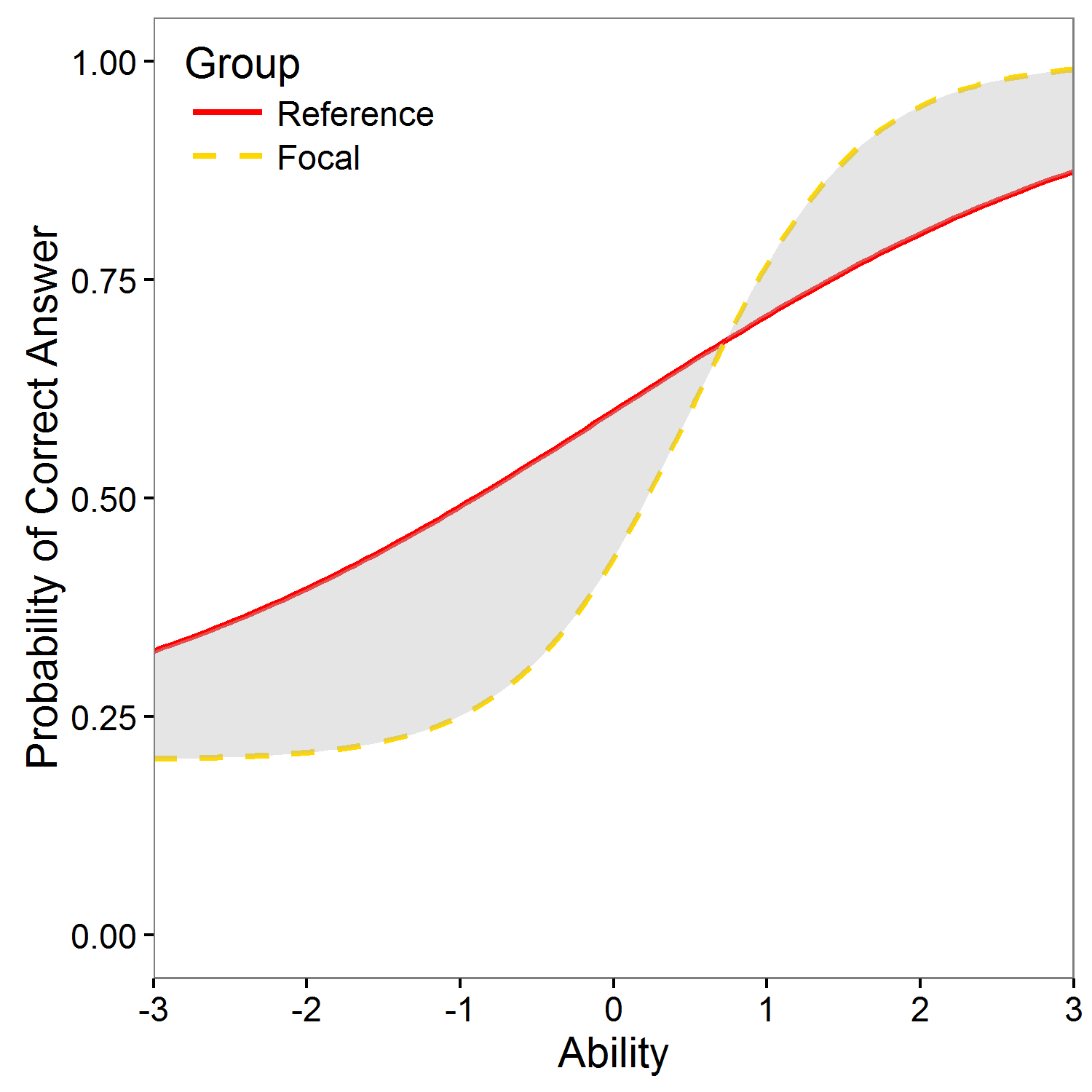
Differential item functioning (DIF) occurs when people from different groups (commonly gender or ethnicity) with the same underlying true ability have a different probability of answering the item correctly. If item functions differently for two groups, it is potentially unfair. In general, two type of DIF can be recognized: if the item has different difficulty for given two groups with the same discrimination, uniform DIF is present (left figure). If the item has different discrimination and possibly also different difficulty for given two groups, non-uniform DIF is present (right figure)
ShinyItemAnalysis
offers an option to download a report in HTML or PDF format. PDF report
creation requires latest version of
MiKTeX
(or other TeX distribution). If you don't have the latest installation, please, use the HTML report.
There is an option whether to use customize settings. By checking the Customize settings local settings will be offered and use for each selected section of report. Otherwise the settings will be taken from pages of application. You can also include your name into report as well as the name of dataset which was used.
Reports by default contain summary of total scores, table of standard scores, item analysis, distractors plots for each item and multinomial regression plots for each item. Other analyses can be selected below.
Validity
Difficulty/discrimination plot
Distractors plots
DIF method selection
Delta plot settings
Logistic regression settings
Multinomial regression settings
Recommendation: Report generation can be faster and more reliable when you first check sections of intended contents. For example, if you wish to include a 3PL IRT model, you can first visit IRT models section and 3PL subsection.
Akaike, H. (1974). A New Look at the Statistical Model Identification. IEEE Transactions on Automatic Control, 19(6), 716-723. See online.
Ames, A. J., & Penfield, R. D. (2015). An NCME Instructional Module on Item-Fit Statistics for Item Response Theory Models. Educational Measurement: Issues and Practice, 34(3), 39-48. See online.
Angoff, W. H., & Ford, S. F. (1973). Item-Race Interaction on a Test of Scholastic Aptitude. Journal of Educational Measurement, 10(2), 95-105. See online.
Bock, R. D. (1972). Estimating Item Parameters and Latent Ability when Responses Are Scored in Two or More Nominal Categories. Psychometrika, 37(1), 29-51. See online.
Cronbach, L. J. (1951). Coefficient Alpha and the Internal Structure of Tests. Psychometrika, 16(3), 297-334. See online.
Drabinova, A., & Martinkova, P. (2016). Detection of Differential Item Functioning Based on Non-Linear Regression. Technical Report V-1229 .
Drabinova, A., & Martinkova, P. (2017). Detection of Differential Item Functioning with Non-Linear Regression: Non-IRT Approach Accounting for Guessing. Journal of Educational Measurement. Accepted.
Lord, F. M. (1980). Applications of Item Response Theory to Practical Testing Problems. Routledge.
Magis, D., & Facon, B. (2012). Angoff's Delta Method Revisited: Improving DIF Detection under Small Samples. British Journal of Mathematical and Statistical Psychology, 65(2), 302-321. See online.
Mantel, N., & Haenszel, W. (1959). Statistical Aspects of the Analysis of Data from Retrospective Studies. Journal of the National Cancer Institute, 22 (4), 719-748. See online.
Martinkova, P., Drabinova, A., & Houdek, J. (2017). ShinyItemAnalysis: Analyza prijimacich a jinych znalostnich ci psychologických testu. TESTFORUM, 6(9), 16–35. See online. (ShinyItemAnalysis: Analyzing admission and other educational and psychological tests)
Martinkova, P., Drabinova, A., Liaw, Y. L., Sanders, E. A., McFarland, J. L., & Price, R. M. (2017). Checking Equity: Why Differential Item Functioning Analysis Should Be a Routine Part of Developing Conceptual Assessments. CBE-Life Sciences Education, 16(2). See online.
Martinkova, P., Stepanek, L., Drabinova, A., Houdek, J., Vejrazka, M., & Stuka, C. (2017). Semi-real-time analyses of item characteristics for medical school admission tests. In: Proceedings of the 2017 Federated Conference on Computer Science and Information Systems. In print.
Swaminathan, H., & Rogers, H. J. (1990). Detecting Differential Item Functioning Using Logistic Regression Procedures. Journal of Educational Measurement, 27(4), 361-370. See online.
Raju, N. S. (1988). The Area between Two Item Characteristic Curves. Psychometrika, 53 (4), 495-502. See online.
Raju, N. S. (1990). Determining the Significance of Estimated Signed and Unsigned Areas between Two Item Response Functions. Applied Psychological Measurement, 14 (2), 197-207. See online.
Rasch, G. (1960) Probabilistic Models for Some Intelligence and Attainment Tests. Copenhagen: Paedagogiske Institute.
Schwarz, G. (1978). Estimating the Dimension of a Model. The Annals of Statistics, 6(2), 461-464. See online.
Wilson, M. (2005). Constructing Measures: An Item Response Modeling Approach.
Wright, B. D., & Stone, M. H. (1979). Best Test Design. Chicago: Mesa Press.
ShinyItemAnalysis
Test and item analysis | Version 1.2.3
![]()
![]()
![]()
© 2017 Patricia Martinkova, Adela Drabinova, Ondrej Leder and Jakub Houdek